Poiseuille Flow and the Hagen–Poiseuille Equation

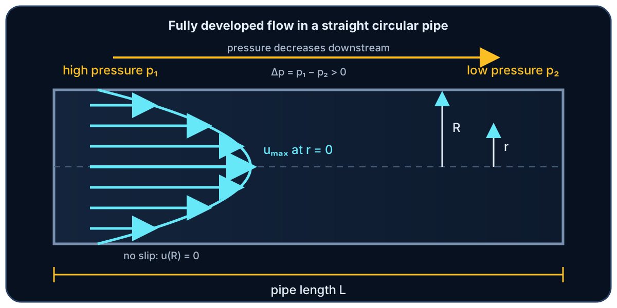
Poiseuille flow is steady, fully developed flow of a Newtonian fluid through a straight circular pipe. If the pressure is higher at the inlet than at the outlet, the velocity is zero at the wall and rises in a parabola to its maximum at the center.

For pipe radius $R$, length $L$, dynamic viscosity $\mu$, and pressure drop $\Delta p=p_{\mathrm{in}}-p_{\mathrm{out}}>0$, the volume flow rate is

$$Q=\frac{\pi R^4\Delta p}{8\mu L}=\frac{\pi D^4\Delta p}{128\mu L}.$$

The axial velocity at distance $r$ from the centerline is

$$u(r)=\frac{\Delta p}{4\mu L}(R^2-r^2)=u_{\max}\left(1-\frac{r^2}{R^2}\right).$$

These formulas are the Hagen–Poiseuille equation, also called Poiseuille's law. They require a steady, incompressible, Newtonian, fully developed flow in a rigid circular pipe with no slip at the wall. Outside that setting, the formula may need correction or may not apply.

Let a straight circular pipe have radius $R$ and axial coordinate $z\in[0,L]$. Write $G=-dp/dz=\Delta p/L>0$ for a constant pressure gradient, where $\Delta p=p_{\mathrm{in}}-p_{\mathrm{out}}$. The Hagen–Poiseuille solution of the incompressible Newtonian Navier–Stokes equations is

$$\mathbf{u}(r)=u_z(r)\mathbf{e}_z,\qquad u_z(r)=\frac{G}{4\mu}(R^2-r^2),$$

with

$$u_{\max}=\frac{GR^2}{4\mu},\qquad \bar{u}=\frac{GR^2}{8\mu}=\frac{u_{\max}}{2},\qquad Q=\pi R^2\bar{u}=\frac{\pi GR^4}{8\mu}.$$

Equivalently, $Q=\pi R^4\Delta p/(8\mu L)=\pi D^4\Delta p/(128\mu L)$. Here $\mu$ is dynamic viscosity; kinematic viscosity is $\nu=\mu/\rho$. The result assumes steady, incompressible, axisymmetric, fully developed flow of a Newtonian fluid in a straight, rigid, constant-radius circular pipe, with a constant effective axial pressure gradient and no slip.

The equation is powerful because it describes a very specific experiment. Imagine a long, straight, rigid tube with a constant circular cross-section. The fluid has settled into the same profile at every downstream location: it is no longer developing from the entrance. Every fluid particle moves parallel to the pipe axis, and the pressure falls uniformly along the pipe.

Calling the flow laminar says that this orderly profile is physically realized, rather than replaced by a disturbed or turbulent state. It does not turn Reynolds number into a universal on/off switch; transition depends on disturbances and the apparatus.

Use cylindrical coordinates $(r,\theta,z)$ and the ansatz

$$\mathbf{u}=u_z(r)\mathbf{e}_z,\qquad p=p(z).$$

Steady means $\partial_t\mathbf{u}=0$; fully developed means $\partial_z u_z=0$; axisymmetry means $\partial_\theta u_z=0$; and there are no radial or azimuthal velocity components. A conservative axial body force, such as uniform gravity along a tilted pipe, can be absorbed into an effective pressure. Without doing that, its axial term must be retained explicitly.

The boundary and regularity conditions are

$$u_z(R)=0,\qquad u_z(0)\text{ finite},\qquad u_z'(0)=0.$$

The no-slip condition supplies the wall value. Finiteness and axisymmetry eliminate a logarithmic integration term at $r=0$. For a finite physical pipe, this profile describes a fully developed region away from entrance and exit effects; it is not the complete inlet-to-outlet solution.

The hard term in Navier–Stokes is self-advection: the fluid carries its own velocity into regions with different velocity. In fully developed Poiseuille flow, the velocity points only down the pipe, but it varies only across the pipe. A particle has no radial velocity with which to carry itself across that variation, and the profile does not change in the direction it travels. The self-advection term is therefore exactly zero.

Pressure pushes downstream while viscosity transmits the wall's resistance inward. Those two effects balance at every radius:

$$0=-\frac{dp}{dz}+\mu\left[\frac{1}{r}\frac{d}{dr}\left(r\frac{du}{dr}\right)\right].$$

With $G=-dp/dz>0$, this is just a second-order ordinary differential equation in $r$. The original nonlinear three-dimensional PDE has become a linear radial problem because the geometry removed the feedback term.

For where the full equation comes from, see the Navier–Stokes derivation. For the governing system being specialized here, see the incompressible Navier–Stokes equations.

For constant density and viscosity, with no unabsorbed body force,

$$\rho\left(\partial_t\mathbf{u}+(\mathbf{u}\cdot\nabla)\mathbf{u}\right)=-\nabla p+\mu\Delta\mathbf{u},\qquad \nabla\cdot\mathbf{u}=0.$$

The field $\mathbf{u}=u_z(r)\mathbf{e}_z$ is divergence-free because $u_r=u_\theta=0$ and $\partial_z u_z=0$. Its material-advection term is

$$(\mathbf{u}\cdot\nabla)\mathbf{u}=u_z(r)\,\partial_z\big(u_z(r)\mathbf{e}_z\big)=0.$$

The radial and azimuthal momentum equations give $\partial_r p=\partial_\theta p=0$. The axial component becomes

$$0=-\frac{dp}{dz}+\mu\left(\frac{d^2u_z}{dr^2}+\frac{1}{r}\frac{du_z}{dr}\right).$$

Defining $G=-dp/dz>0$ gives

$$\frac{1}{r}\frac{d}{dr}\left(r\frac{du_z}{dr}\right)=-\frac{G}{\mu}.$$

This cancellation is exact for the ansatz; it is not an approximation that discards inertia on the basis of small Reynolds number.

Start with the reduced equation and multiply by $r$:

$$\frac{d}{dr}\left(r\frac{du}{dr}\right)=-\frac{G}{\mu}r.$$

Integrate once. Symmetry rules out a singular term at the center, leaving

$$\frac{du}{dr}=-\frac{G}{2\mu}r.$$

Integrate again:

$$u(r)=-\frac{G}{4\mu}r^2+C.$$

No slip says $u(R)=0$, so $C=GR^2/(4\mu)$. Therefore

$$u(r)=\frac{G}{4\mu}(R^2-r^2).$$

The curve is a parabola. It is zero at $r=R$, symmetric about the centerline, and largest at $r=0$. In normalized form, the entire family has the same shape:

$$\frac{u(r)}{u_{\max}}=1-\left(\frac{r}{R}\right)^2.$$

Integrating

$$\frac{d}{dr}(ru_z')=-\frac{G}{\mu}r$$

gives

$$ru_z'=-\frac{G}{2\mu}r^2+C_1,\qquad u_z'=-\frac{G}{2\mu}r+\frac{C_1}{r}.$$

If $C_1\ne0$, a second integration produces $C_1\log r$, which is singular on the pipe axis. Centerline regularity therefore forces $C_1=0$. A second integration yields

$$u_z(r)=-\frac{G}{4\mu}r^2+C_2.$$

The no-slip condition $u_z(R)=0$ fixes $C_2=GR^2/(4\mu)$, hence

$$u_z(r)=\frac{G}{4\mu}(R^2-r^2).$$

It follows directly that $u_z'(0)=0$ and $u_{\max}=u_z(0)=GR^2/(4\mu)$. With $\hat r=r/R$ and $\hat u=u_z/u_{\max}$, the dimensionless profile is $\hat u=1-\hat r^2$.

The velocity profile tells us how fast each circular ring of fluid moves. Add those rings across the cross-section:

$$Q=\int_Au\,dA=\int_0^R u(r)\,2\pi r\,dr=\frac{\pi R^4\Delta p}{8\mu L}.$$

Dividing by the cross-sectional area gives the mean speed, which is exactly half the centerline speed:

$$\bar u=\frac{Q}{\pi R^2}=\frac{\Delta p R^2}{8\mu L}=\frac{u_{\max}}{2}.$$

The same equation can be written as a pressure–flow resistance law:

$$\Delta p=\mathcal{R}_hQ,\qquad \mathcal{R}_h=\frac{8\mu L}{\pi R^4}.$$

This resembles Ohm's law: pressure drop plays the role of voltage, volume flow plays the role of current, and $\mathcal{R}_h$ is hydraulic resistance. The analogy is exact only while the linear Poiseuille assumptions hold.

Viscous shear is largest in magnitude at the wall:

$$|\tau_w|=\frac{\Delta p R}{2L}.$$

For an axisymmetric profile, $dA=2\pi r\,dr$, so

$$Q=2\pi\int_0^R\frac{G}{4\mu}(R^2-r^2)r\,dr=\frac{\pi GR^4}{8\mu}.$$

Thus

$$\bar u=\frac{Q}{\pi R^2}=\frac{GR^2}{8\mu},\qquad u_{\max}=2\bar u.$$

Substituting $G=\Delta p/L$ gives both common forms:

$$Q=\frac{\pi R^4\Delta p}{8\mu L}=\frac{\pi D^4\Delta p}{128\mu L},\qquad \Delta p=\frac{128\mu LQ}{\pi D^4}.$$

The shear component is

$$\tau_{rz}=\mu\frac{du_z}{dr}=-\frac{G}{2}r.$$

Its sign indicates that viscous traction opposes the downstream motion; its wall magnitude is $|\tau_w|=GR/2=\Delta pR/(2L)$. The hydraulic resistance $\mathcal{R}_h=8\mu L/(\pi R^4)$ applies to the specified circular tube and linear regime, not to arbitrary ducts or turbulent networks.

Take a water-like Newtonian fluid with $\mu=1.00\times10^{-3}\,\mathrm{Pa\,s}$ in a pipe of radius $R=1.00\,\mathrm{mm}$ and length $L=1.00\,\mathrm{m}$. Apply a pressure drop $\Delta p=1.00\,\mathrm{kPa}$.

Convert millimeters to meters before taking the fourth power: $R=1.00\times10^{-3}\,\mathrm{m}$, so $R^4=1.00\times10^{-12}\,\mathrm{m^4}$. Then

$$Q=\frac{\pi(1.00\times10^{-3})^4(1.00\times10^3)}{8(1.00\times10^{-3})(1.00)}=3.93\times10^{-7}\,\mathrm{m^3/s}.$$

That is $0.393\,\mathrm{mL/s}$. The mean speed is

$$\bar u=\frac{Q}{\pi R^2}=0.125\,\mathrm{m/s},$$

and the centerline speed is $u_{\max}=0.250\,\mathrm{m/s}$. Using $\rho=1000\,\mathrm{kg/m^3}$ gives $\mathrm{Re}_D=\rho\bar uD/\mu=250$, consistent with an orderly laminar realization in a smooth, well-controlled pipe.

The units are a useful error check: $R^4\Delta p/(\mu L)$ reduces to $\mathrm{m^3/s}$.

With $\mu=10^{-3}\,\mathrm{Pa\,s}$, $R=10^{-3}\,\mathrm{m}$, $L=1\,\mathrm{m}$, and $\Delta p=10^3\,\mathrm{Pa}$,

$$G=\frac{\Delta p}{L}=10^3\,\mathrm{Pa/m},\qquad Q=\frac{\pi GR^4}{8\mu}=3.927\times10^{-7}\,\mathrm{m^3/s}.$$

Since $A=\pi R^2=3.142\times10^{-6}\,\mathrm{m^2}$,

$$\bar u=0.125\,\mathrm{m/s},\qquad u_{\max}=0.250\,\mathrm{m/s},\qquad |\tau_w|=\frac{GR}{2}=0.500\,\mathrm{Pa}.$$

For $\rho=1000\,\mathrm{kg/m^3}$ and $D=2R=2\times10^{-3}\,\mathrm{m}$, $\mathrm{Re}_D=250$. The dimensional check is

$$\frac{[R]^4[\Delta p]}{[\mu][L]}=\frac{\mathrm{m^4}(\mathrm{kg\,m^{-1}s^{-2}})}{(\mathrm{kg\,m^{-1}s^{-1}})\mathrm{m}}=\mathrm{m^3/s}.$$

The input values are illustrative rather than a calibrated prediction for a particular device.

At fixed pressure drop, length, and viscosity, doubling the radius multiplies $Q$ by $2^4=16$. Halving the radius cuts the flow rate to $1/16$. This extreme sensitivity is the best-known feature of Poiseuille's law.

Two factors combine to create $R^4$. A wider pipe has more area, contributing roughly $R^2$. It also lets the velocity parabola become taller: the mean speed itself grows like $R^2$. Area times mean speed gives $R^4$.

The law is useful for estimating resistance in circular capillaries, designing laminar-flow experiments, and interpreting capillary viscometers. Similar pressure–flow ideas guide microfluidics, but many microchannels are rectangular rather than circular, so their conductance coefficient is different.

Biological flow needs special care. The formula can be an approximation in restricted small-vessel settings, but blood may be non-Newtonian, flow may pulse, and vessel walls may deform. It is not a complete model of an artery, and the equation alone should not be used for a medical conclusion.

From

$$Q=\frac{\pi\Delta p}{8\mu L}R^4,$$

the logarithmic sensitivities are $\partial\log Q/\partial\log R=4$, $\partial\log Q/\partial\log\Delta p=1$, $\partial\log Q/\partial\log\mu=-1$, and $\partial\log Q/\partial\log L=-1$, provided the other variables and the model regime are held fixed.

The $R^4$ dependence factors as $Q=A\bar u$, with $A\sim R^2$ and $\bar u\sim GR^2/\mu$. Changing $R$ can also change $\mathrm{Re}_D$: at fixed $G$, $\bar u\sim R^2$ and $D\sim R$, so $\mathrm{Re}_D\sim R^3$. A sufficiently large radius change can therefore invalidate the laminar physical realization before an extrapolated $R^4$ prediction is reached.

For non-circular ducts, pressure-driven fully developed flow still gives a linear conductance relation for a Newtonian fluid, but the geometric factor comes from solving a cross-sectional Poisson problem; one cannot simply insert a hydraulic radius into the circular $R^4$ formula and expect an exact result.

Before using the equation, check the physical problem against its assumptions.

• Near the entrance: the profile is still developing and has a radial component, so the fully developed solution is incomplete.
• Disturbed or turbulent pipe flow: a parabolic laminar profile may not be the observed state. A diameter Reynolds number around 2,300 is a common engineering guide, not a universal theorem.
• Non-Newtonian fluids: shear-thinning, shear-thickening, yield-stress, and other rheologies produce different profiles and pressure–flow laws.
• Strongly unsteady or pulsatile flow: inertia introduces time dependence and phase lag; an instantaneous steady formula can miss the dynamics.
• Compressible flow: significant density changes along the pipe require mass-flow and thermodynamic relations.
• Different boundaries or geometry: wall slip, porous walls, curved or tapered pipes, non-circular ducts, and deforming walls change the problem.

In the ideal fully developed model, the parabolic field remains an exact steady Navier–Stokes solution for any parameter value. What changes with Reynolds number is whether that state persists under real disturbances and describes the observed flow. Learn more in Reynolds number and turbulence.

The often-quoted $\mathrm{Re}_D\approx2300$ is an engineering transition convention, not a sharp existence boundary for the formula. Here

$$\mathrm{Re}_D=\frac{\rho\bar uD}{\mu}=\frac{\bar uD}{\nu}.$$

The Hagen–Poiseuille field is an exact solution of the ideal fully developed equations even when the numerical Reynolds number is larger. Transition concerns stability, finite disturbances, inlet conditions, wall roughness, and whether the laminar solution is physically realized. Consequently, the right validation question is not only Is Re below 2300? but also whether the geometry, constitutive law, boundary conditions, development length, and disturbance environment match the model.

For unsteady pressure gradients in a rigid circular pipe, the Womersley problem replaces the steady profile. Generalized Newtonian fluids change the constitutive relation between $\tau_{rz}$ and $du_z/dr$. Compressible flows couple density to pressure and temperature. Non-circular cross-sections replace the radial ODE with a two-dimensional Poisson problem. Each is a different reduction, not a correction that can always be hidden inside $\mu$ or $R$.

For fully developed laminar flow in a circular pipe, Poiseuille's law and the Darcy–Weisbach pressure-loss equation say the same thing in different notation. Using mean speed $\bar u$ and diameter $D$,

$$\Delta p=f_D\frac{L}{D}\frac{\rho\bar u^2}{2},\qquad f_D=\frac{64}{\mathrm{Re}_D}.$$

Here $f_D$ is the Darcy friction factor. The Fanning friction factor is four times smaller, $16/\mathrm{Re}_D$, which is a common source of factor-of-four errors.

This exact solution also clarifies what is and is not unsolved about Navier–Stokes. We have solved this highly symmetric steady flow completely. We have not proved that every smooth three-dimensional incompressible initial flow stays smooth forever. Poiseuille geometry removes the nonlinear self-advection that drives the general difficulty.

Continue with the catalog of exact Navier–Stokes solutions, or see the existence-and-smoothness problem for the statement that remains open.

From Poiseuille's law, $\Delta p=32\mu L\bar u/D^2$. Equating this with the Darcy–Weisbach form

$$\Delta p=f_D\frac{L}{D}\frac{\rho\bar u^2}{2}$$

gives

$$f_D=\frac{64\mu}{\rho\bar uD}=\frac{64}{\mathrm{Re}_D}.$$

This is the Darcy friction factor for a fully developed laminar Newtonian flow in a circular pipe; the Fanning convention gives $f_F=f_D/4=16/\mathrm{Re}_D$.

The derivation succeeds because the invariant ansatz $\mathbf{u}=u_z(r)\mathbf{e}_z$ annihilates $(\mathbf{u}\cdot\nabla)\mathbf{u}$ and reduces the PDE to a coercive radial boundary-value problem. The Clay problem quantifies over broad classes of smooth divergence-free three-dimensional data whose evolution has no such symmetry. One explicit global solution neither proves global regularity for all admissible data nor constructs a breakdown example.

What is the Hagen–Poiseuille equation?
The volume flow rate through a straight circular pipe is $Q=\pi R^4\Delta p/(8\mu L)$ under steady, incompressible, Newtonian, fully developed, no-slip conditions.

Why is Poiseuille flow parabolic?
A constant pressure gradient balances viscous diffusion. In a circular pipe, integrating the radial Laplacian twice and applying centerline symmetry plus no slip produces $u(r)\propto R^2-r^2$.

What is the relation between maximum and average velocity?
For the circular-pipe Poiseuille profile, $u_{\max}=2\bar u$.

Why does flow rate depend on radius to the fourth power?
Cross-sectional area contributes a factor $R^2$, while the mean speed also grows like $R^2$ at fixed pressure gradient and viscosity. Their product gives $Q\propto R^4$.

Does Poiseuille's law apply to blood flow?
Only as a limited approximation when the rigid-tube, Newtonian, steady, fully developed assumptions are reasonable. Pulsatility, vessel compliance, branching, and non-Newtonian behavior can all matter.

What is the Hagen–Poiseuille equation?
For the stated circular-pipe assumptions, $Q=\pi R^4\Delta p/(8\mu L)=\pi D^4\Delta p/(128\mu L)$ and $u_z(r)=\Delta p(R^2-r^2)/(4\mu L)$.

Why is Poiseuille flow parabolic?
The axial equation $r^{-1}(ru_z')'=-G/\mu$ integrates to a quadratic once the singular $\log r$ mode is excluded and $u_z(R)=0$ is imposed.

What is the relation between maximum and average velocity?
Area integration gives $\bar u=GR^2/(8\mu)$ while $u_{\max}=GR^2/(4\mu)$, hence $u_{\max}=2\bar u$.

Why does flow rate depend on radius to the fourth power?
At fixed $G$ and $\mu$, the cross-sectional scale is $R^2$ and the velocity scale is $GR^2/\mu$, giving $Q\sim GR^4/\mu$.

Does Poiseuille's law apply to blood flow?
It can serve as a local idealization, not a universal hemodynamic law. A defensible use must assess non-Newtonian rheology, pulsatility, compliance, branching, and development effects.